Treatment of boundaries in Markov chain Monte Carlo
I have been asked by multiple students what to do with MCMC at boundaries, in particular how to treat proposals that lie outside the support of the target. Suppose we have a vector of parameters \(\theta\) and want to target a density (proportional to) \(\pi(\theta)\) using a proposal distribution \(q(\theta'|\theta)\). In MCMC, we seek to define a Markov process in discrete time, \((\theta_0, \theta_1, \ldots, \theta_N)\) that has stationary distribution with density \(\pi\). In the Metropolis Hastings scheme, the law of such a process is that at step \(m\), when the state of the system is \(\theta_m\), we pick a proposed new value \(\tilde{\theta}\) with density \(q(\cdot | \theta_m)\), then
The natural question is, if there is somewhere we can propose but not move (e.g. because the likelihood is not defined) then what should be done?
Let us consider one parameter, a probability \(p\in [0,1]\), with a density \(\pi(p) = \mathrm{Uniform}(0,1)\), and a proposal distribution \(q(p'|p) = \mathcal{N}(p'|p,1)\). We will run chains of length \(N=10^7\). Code is all in R.
In the first chain (‘Keep picking’) we will keep proposing new values until one is within the allowed region
In the second chain (‘Reject’) we will reject proposals outside the region and remain at the position the proposal was made.
Now look at some plots
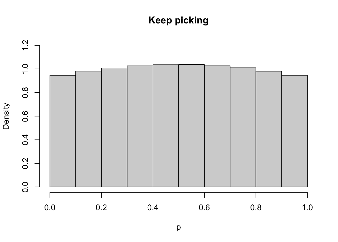
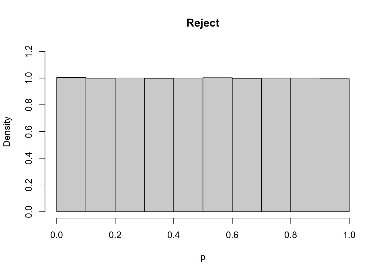
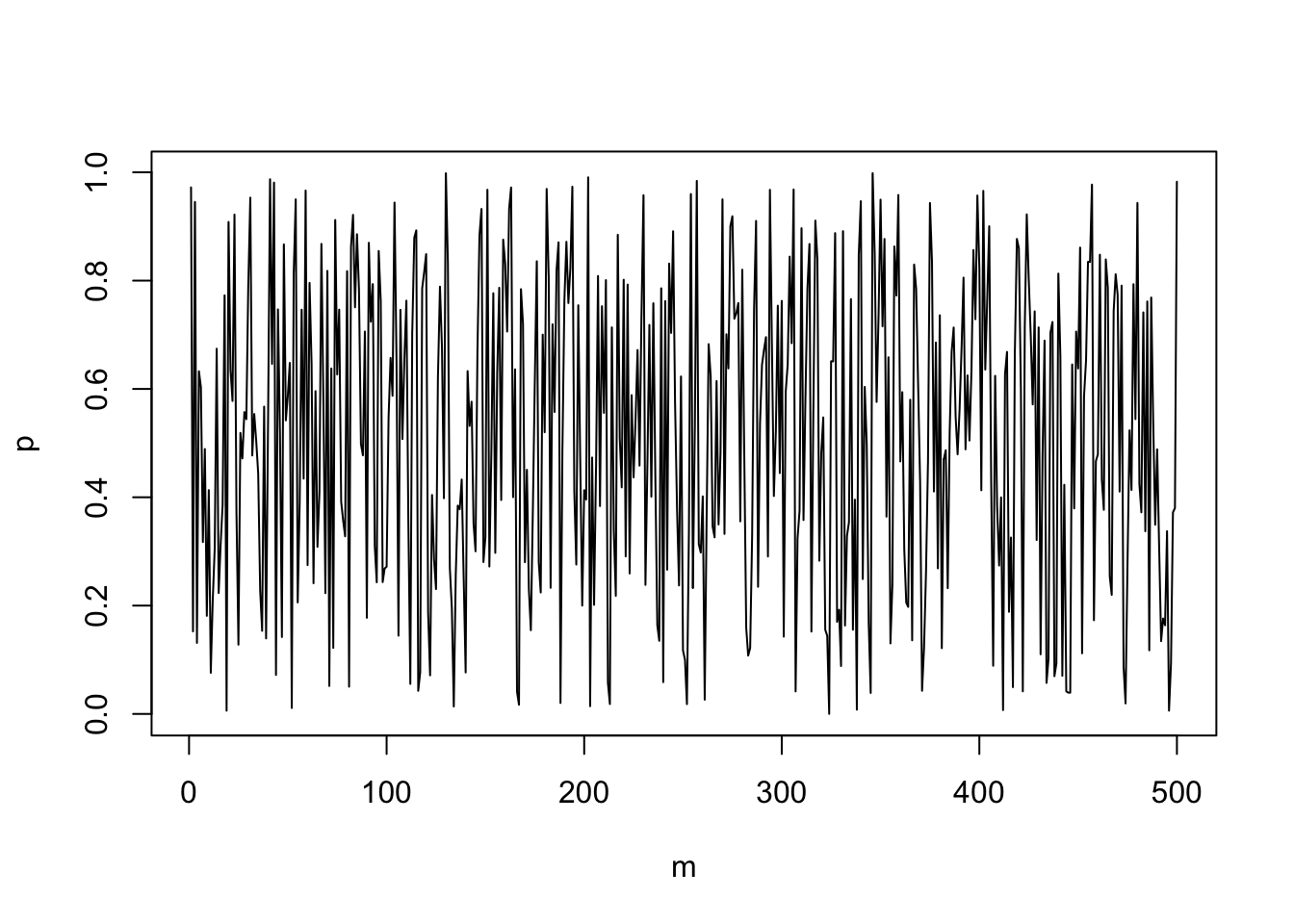
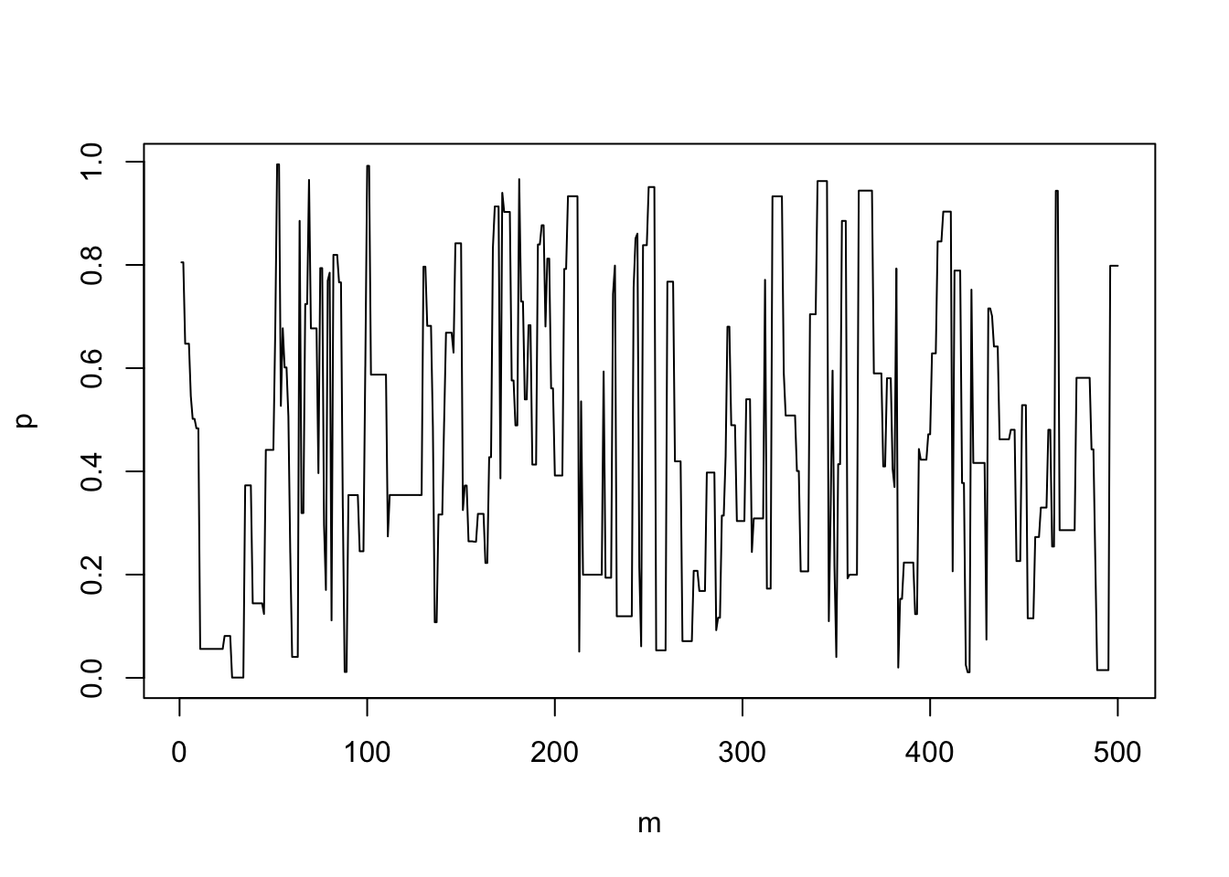
What we see is that the first approach, the trace plot looks superficially ‘better’, but the output is biased. From the Metropolis-Hastings algorith as specified in \((\dagger)\) this is what we would expect; mathematically, we can interpret the ‘Reject’ approach as taking \(\pi(\theta<0) = \pi(\theta>1) = 0\), while the ‘Keep picking’ approach the proposal distribution effectively becomes a truncated normal. Such a truncated normal could be evaluated as the \(q(\cdot|\cdot)\) in \((\dagger)\), and this might be a good algorithm, but the naïve implementation introduces bias.